Computing the boundary complex using Macaulay2

2023-05-08

Suppose you are given a divisor $D$ on a variety $X$ , with $D = \cup_{i = 0}^{N} D_{i}$ the decomposition into its irreducible components. Suppose moreover that the divisor is simple normal crossing, or even combinatorial normal crossing in the sense that all non-empty intersections $D_{i_{1}} \cap . . . \cap D_{i_{k}}$ have codimension $k$ . One can form the boundary complex $Δ (D)$ of $D$ , a simplicial complex on the set $0, . . ., N$ recording the intersection properties of the $D_{i}$ . We proceed as follows:

For each $D_{i}$ , add a vertex $[i]$ to the complex $Δ (D)$ .
For each non-empty intersection $D_{i_{1}} \cap . . . \cap D_{i_{k}}$ , add a k-simplex $[i_{1}, . ., i_{k}]$ between the vertices $[i_{1}]$ , $[i_{2}]$ ,... through to $[i_{k}]$ .

From this boundary complex, interesting information about the divisor $D$ and its complement $U := X ∖ D$ can be deduced.

When working in the projective plane $P^{2}$ , we might have a divisor $D$ given as the union of curves $D_{0}, . . ., D_{N}$ , each given by a corresponding irreducible polynomials $f_{i}$ . Suppose we are given this list of polynomials $f_{0}, . . ., f_{N}$ .

Here is some Macaulay2 code that will compute the boundary complex in this case:

boundaryComplex = method()
boundaryComplex := listOfDivisors -> (
-- Helper function, takes list of polynomials and determines 
-- if their intersection is irrelevant ideal
intersectionIsIrrelevantIdeal = s -> (
radical(ideal(s)) != ideal(y_0,y_1,y_2)
);
-- Select all possible subsets of divisors
rawPolySubs = subsets(listOfDivisors);
polySubs = rawPolySubs_{1..(#rawPolySubs-1)};
-- Create a true/false mask for when this intersection is the irrelevant 
-- ideal and hence those divisors do not intersect in projective space
mask = apply(polySubs,intersectionIsIrrelevantIdeal);
-- List all faces
R=QQ[x_0..x_(#listOfDivisors-1)];
-- take subsets of numbers 0 through length(listOfDivisors), then 
-- drop the first as it is always the empty set
faceNums = drop(subsets(toList(0..(#listOfDivisors-1))),1); 
faceSubs = drop(subsets(toList(x_0..x_(#listOfDivisors-1))),1);
-- Filter by the mask
faceMonomials = {};
faceList = {};
for i in 0..(#faceSubs-1) do (
    if mask#i then (
        faceMonomials=append(faceMonomials,fold((i,j)->i*j, faceSubs#i));
        faceList=append(faceList,faceNums#i);
    )
);
(simplicialComplex(faceMonomials),faceList))

The function outputs two objects:

First, a SimplicialComplex object, which is exactly $Δ (D)$ , and can be easily visualized (see below).
Second, a list of the faces of this simplicial complex as subsets of the integers $0, . ., N$ , which can be useful for a quick inspection and building the simplicial complex in some other program, such as Polymake

It should be a straightforward matter to generalize this to divisors on other varieties, say in the toric setting, by changing the irrelevant ideal $(y_{0}, y_{1}, y_{2})$ on line 6 to another ideal.

An example run of this code is given as follows:


S = QQ[y_0..y_2]
l0 = y_0
l1 = 2*y_1-y_2+y_0
l2 = y_2
c1 = y_0*y_1 + y_0*(y_2 - y_0) + y_1*(y_2 - y_1)
c2 = y_0*y_1 + y_0*(y_2 - 3*y_0) + 3*y_1*(y_2 - 3*y_1)
listOfDivisors = {l0,l1,l2,c1,c2}

(bc, lf) = boundaryComplex(listOfDivisors)

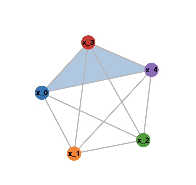
Moreover, using the Visualize package, we can quite easily visualize two-dimensional simplicial complexes (three-dimensional are per now not supported). In the above example this would proceed as follows:


loadPackage "Visualize"
openPort("8090")

visualize bc

closePort()

(Remember to close the port after you are done, if you forget, you might need to use lsof -i tcp:8090 and kill the process holding onto the port).

This should give you a nice interactive browser animation, looking similar to the following image:

For three-dimensional simplicial complexes, the following code will transform the list lf into a string which can be pasted in polymake to create the corresponding polymake simplicial object:


facesToPolymakeSimplicialComplex = method()
facesToPolymakeSimplicialComplex := lst -> (
listStr = toString(lst);
listStr = replace("{","[",listStr);
listStr = replace("}","]",listStr);
out = concatenate({"$s = new SimplicialComplex(INPUT_FACES=>",  listStr, ");"});
out
)

facesToPolymakeSimplicialComplex(lf)

This can then be visualized using the command $s->VISUAL;

Bibliography:

Grayson, Daniel R. and Stillman, Michael E., Macaulay2, a software system for research in algebraic geometry, http://www.math.uiuc.edu/Macaulay2//
Ewgenij Gawrilow and Michael Joswig, polymake: a framework for analyzing convex polytopes, https://polymake.org/doku.php/startt